Introduction to Inferential Statistics
Inferential statistics helps researchers come to conclusions and make predictions based upon their sample data. There are two main uses for inferential statistics: making estimates about populations and drawing conclusions about populations by testing hypotheses. This section will introduce the different types of inferential statistics methods available and explore why there is always a degree of uncertainty due to the error introduced by sampling.
Levels of Measurement
Before we start, here is a reminder of the levels of measurement. Levels of measurement tell you how precisely variables are recorded. There are four levels of measurement. They are described below from lowest to highest precision.
Nominal
This data can only be categorised. Data is given mutually exclusive labels and there is no order between categories. An example is car brands.
Ordinal
This data can be categorised and ranked. You cannot say anything about the intervals between the rankings. An example is language ability.
Interval
This data can be categorised, ranked and evenly spaced. There is no true zero point with different scales giving different zero points. An example is temperature in Fahrenheit or Celsius.
Ratio
This data can be categorised, ranked, evenly spaced and has a true zero point. An example is temperature in Kelvin.
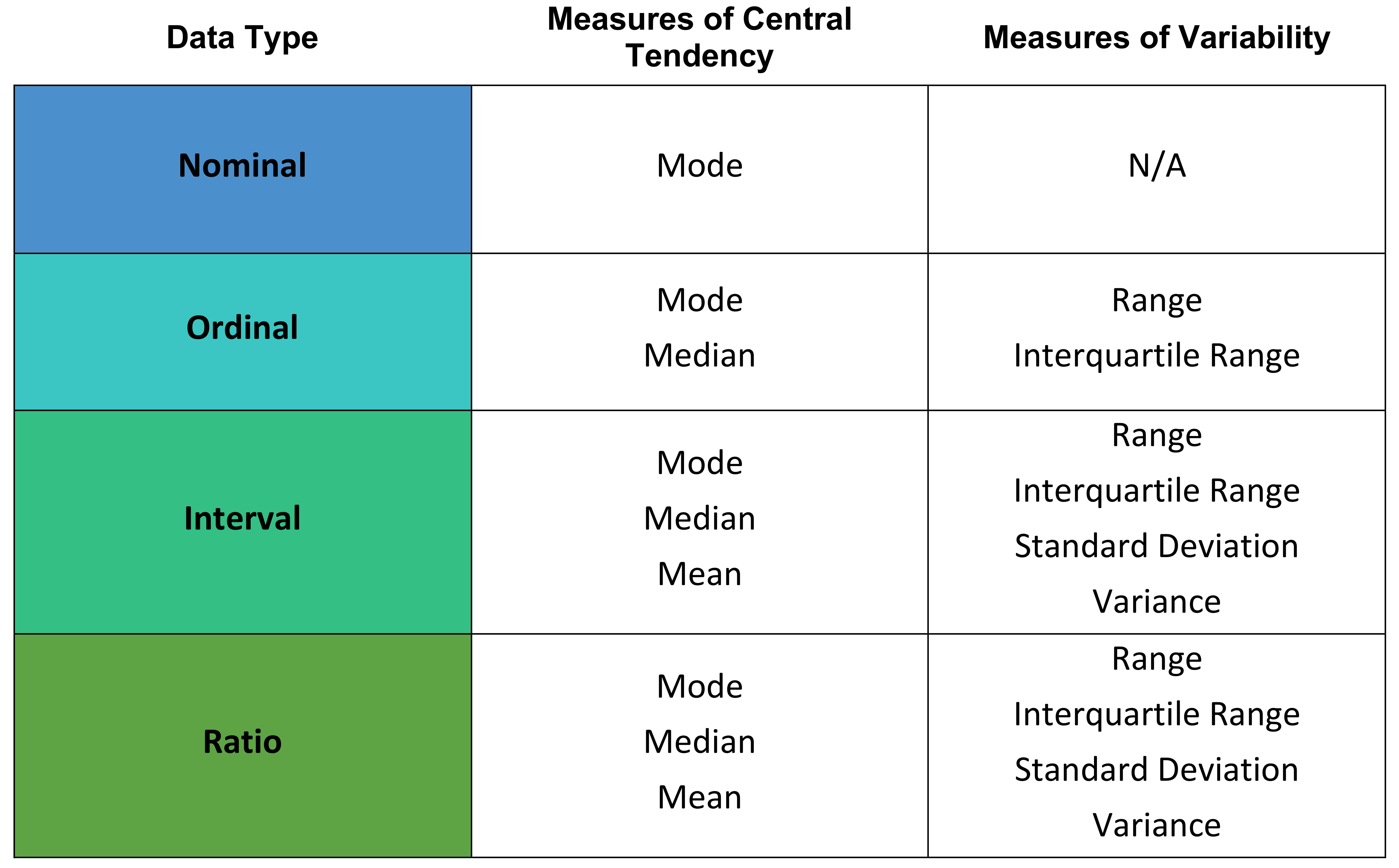
Summary of Descriptive Statistics
The following table provides a summary of descriptive statistics. You can read more about how the level of measurement relates to central tendancy and variability in our article Introduction to Descriptive Statistics.
Standard Error
A parameter is a number that describes a whole population. A statistic is a number that describes a sample. The aim of research is to understand the population by finding parameters through analysing data collected from samples. To make unbiased estimates, your sample should be representative of your population and ideally randomly selected with unbiased sampling methods.
Sampling errors (the difference between a population parameter and a sample statistic) arise any time you gather data using a sample. This is because the sample is always smaller than the size of the population and will not completely reflect the population. The standard error of the mean estimates the variability across multiple samples taken from a population and is a common way to measure the sampling error. In other words, the standard error is used to describe how well your sample data represents the whole population.
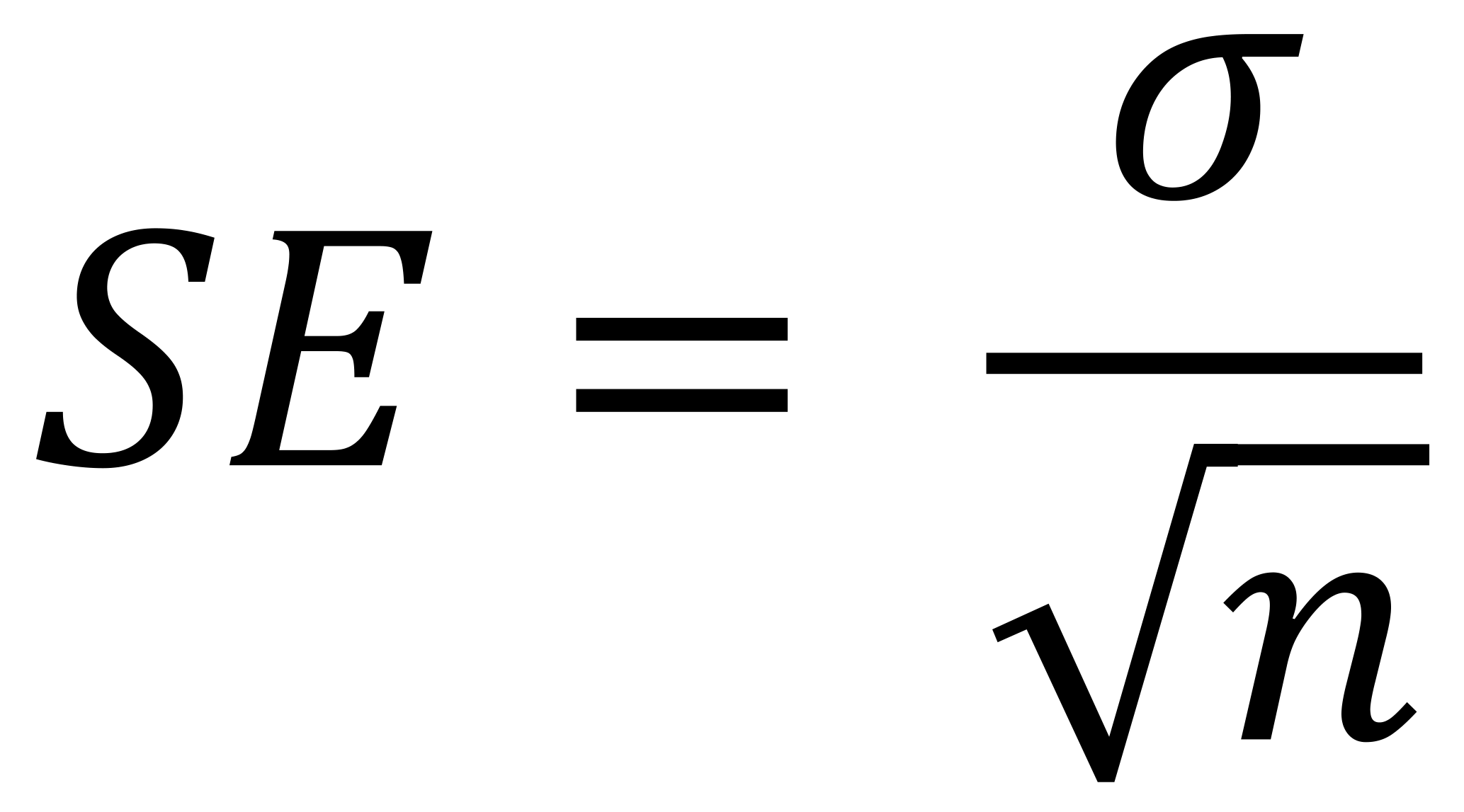
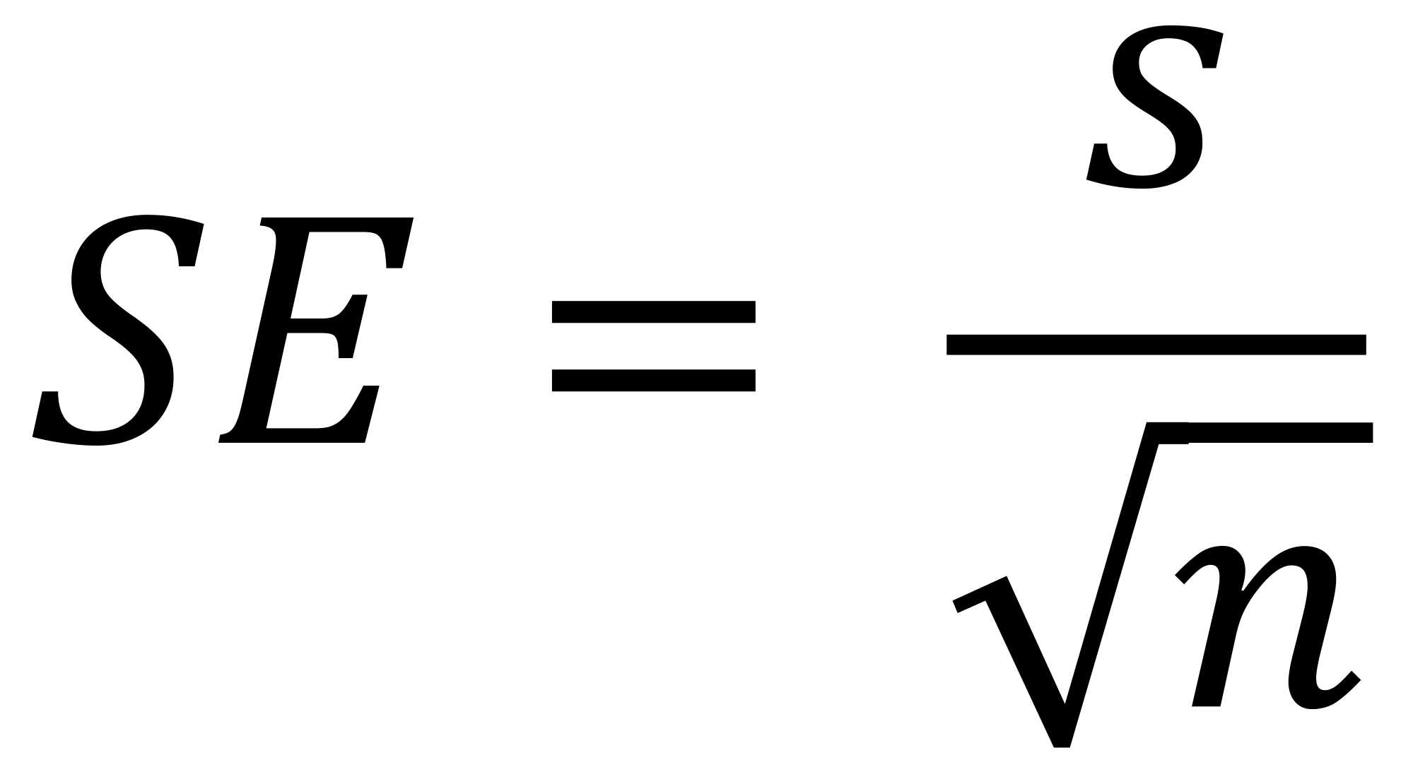
A high standard error shows that the sample means are widely spaced around the population true mean. A low standard error shows that the sample means are closely distributed around the population mean and are therefore likely to be representative of the population. The standard error can be reduced by increasing the sample size. The formula for standard error of the mean will vary depending upon whether the population parameters are known. These formulas will work with samples that contain more than 20 elements. They are as follows:
Known Population Parameters - This will precisely calculate the standard error and where σ is the population standard deviation.
Unknown Population Parameters - This will provide an estimate of the standard error and where s is the sample standard deviation.
Reporting the Standard Error
The standard error can be reported alongside the mean or in a confidence interval to communicate the uncertainty around the mean. For a normally distributed population, a 95% confidence interval would expect 95% of sample means to lie within ± 1.96 standard errors of the mean. For example, where the mean is 200 and the standard error is 10:
- The mean score is 200 ± 10 (SE).
- The 95% confidence interval is 181 to 219.
Estimating Population Parameters
There are two major types of estimate you can make about the population using sample data. They are as follows:
- Point Estimate – this is a single value estimate of the parameter. An example would be using the sample mean as an estimate for the population mean.
- Interval Estimate – this is a range of values where the parameter is expected to lie. An example would be a confidence interval in which you would expect to find the population mean.
It is best to use a combination of point estimates and interval estimates when reporting population characteristics from sample data.
Confidence Intervals
In order to get a true parameter value from the population, you would have to collect data from the entire population. A confidence interval provides an estimate of the population parameter by including the uncertainty introduced by the sampling error. Each confidence interval is associated with a confidence level which tells you the probability of that interval containing the population parameter estimate if you were to re-sample the population again. For example, if you have a confidence interval of 95% you would be confident that 95 out of 100 times the parameter estimate will fall within the limits specified by the confidence interval. You can calculate the confidence interval if you know:
- The population point estimate. For example, the population mean.
- The critical values for the test statistic. This tells you how many standard deviations away from the mean you need to go in order to reach the desired confidence level.
- Choose your alpha value (P-Value).
- Decide if using a one-tailed or two-tailed test.
- Look up the critical value that corresponds with the alpha value. If normally distributed and ≥ 30 samples, you can use the z-distribution. If normally distributed and <30 samples, you can use the t-distribution to correct for small sample sizes.
- The standard deviation of the sample.
- The sample size.
For non-normally distributed data, it is possible to create confidence intervals by either transforming the data to make it fit a normal distribution or by finding a distribution that matches the shape of your data. Calculating the confidence interval for the mean of normally distributed data can be completed using the following formulas:
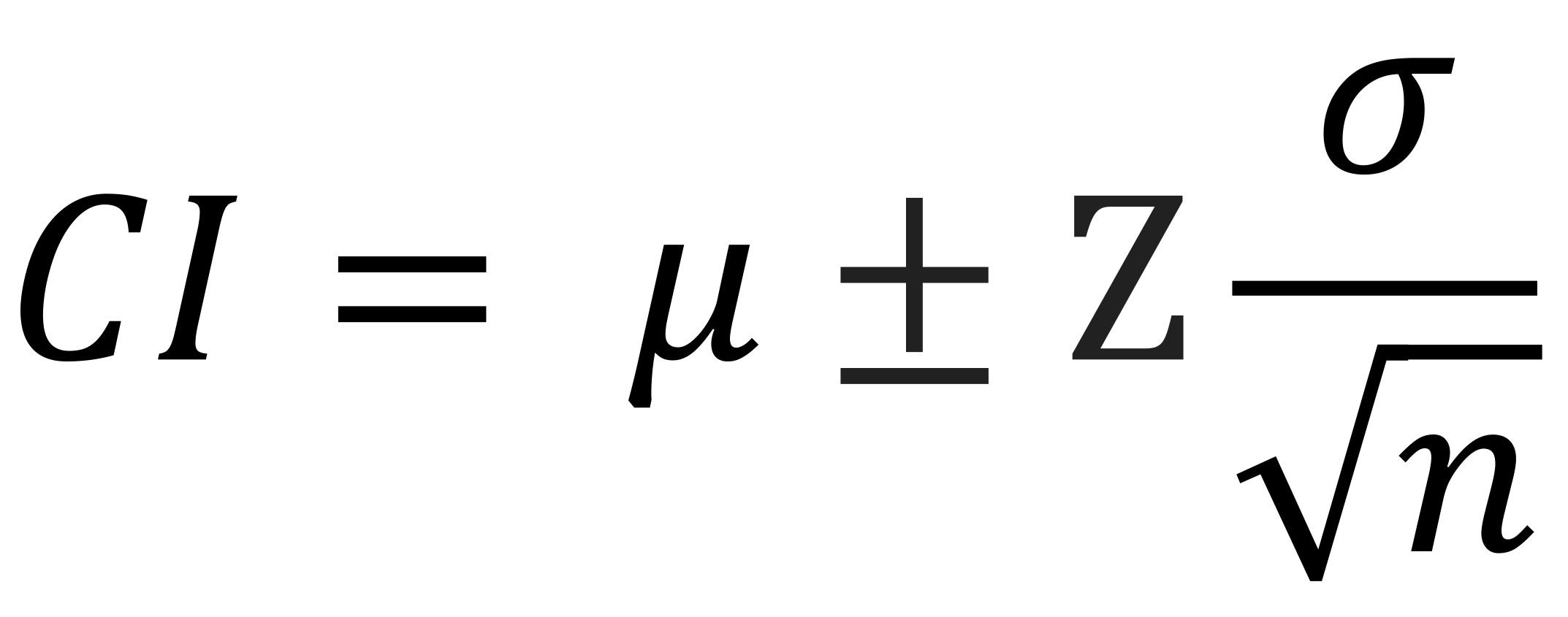
Known Population Parameters - Uses the population mean and standard deviation where μ is the population mean, Z is the critical value and σ is the population standard deviation.
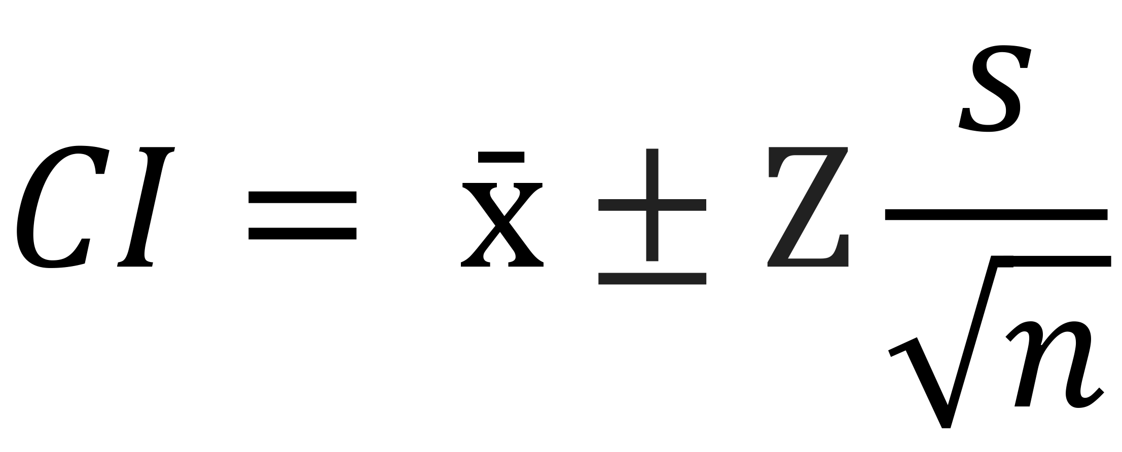
Unkown Population Parameters - Uses the sample mean and standard deviation where x̄ is the sample mean, Z is the critical value and s is the sample standard deviation.
Drawing Conclusions with Hypothesis Testing
A hypothesis is a prediction which is tested using statistical tests in a process known as hypothesis testing. The goal is to use sample data to compare different populations with one another or assess relationships between variables within one population. There are five steps in hypothesis testing:
- State your null hypothesis (H0) and the opposite alternate hypothesis (H1).
- Collect sample data which is representative of the population and is designed to test the hypothesis.
- Perform an appropriate statistical test. This will either be based on the comparison of within-group variance (spread within a category) or the comparison between-group variance (spread between categories).
- Decide whether the null hypothesis (H0) is supported or refuted.
- Present the findings in your results and discussion.
The choice of statistical test largely lies with the sample data you are testing. It will be influenced by the level of measures used when gathering data and whether the data is parametric or non-parametric. There are three broad categories of tests you can use: comparison, correlation or regression. For further information on interpretation of hypothesis testing, please see the article on P-Values.
Parametric Test Assumptions
- The population follows a normal distribution of scores.
- The sample data is independent and representative of the population.
- The variances of each comparison group are similar.
Non-Parametric Tests
- These should be performed for any data which does not uphold the parametric assumptions.
- They are “distribution-free tests” because they assume nothing about the distribution of the population data.
- The inferences made by non-parametric tests are not as strong as the inferences made by parametric tests.
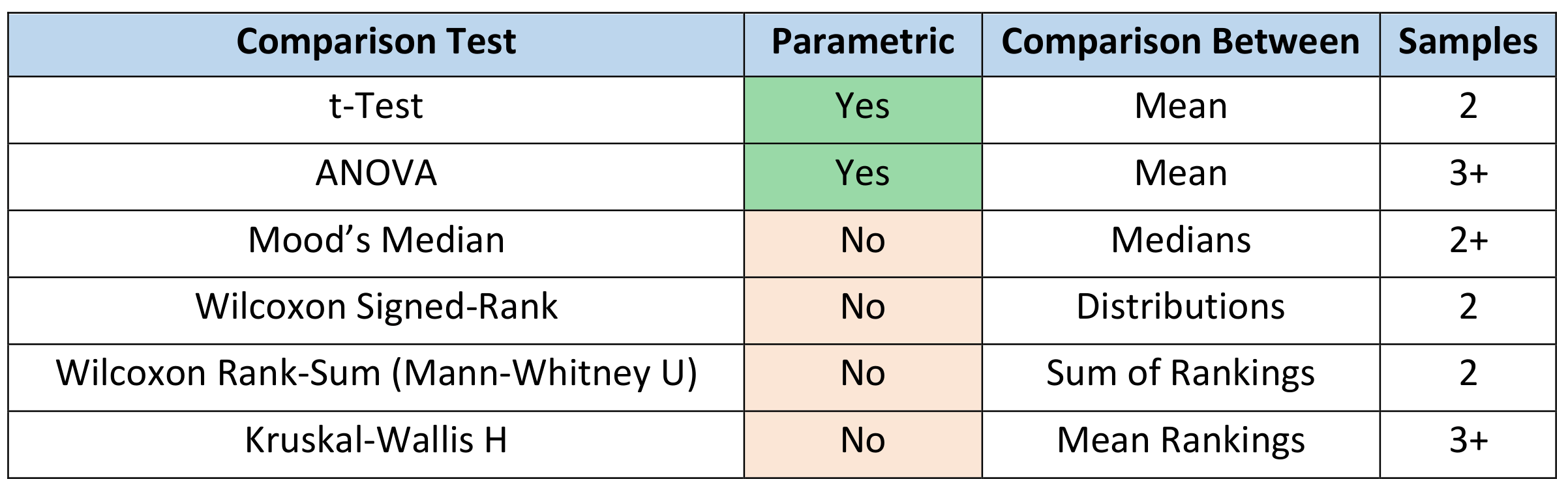
Comparison Tests
These assess whether there are differences in the means, medians or rankings of score between two or more groups. The type of test you select will depend upon whether your data is parametric, the number of samples and the levels of measurement of your variables. The tests you can employ are as follows:
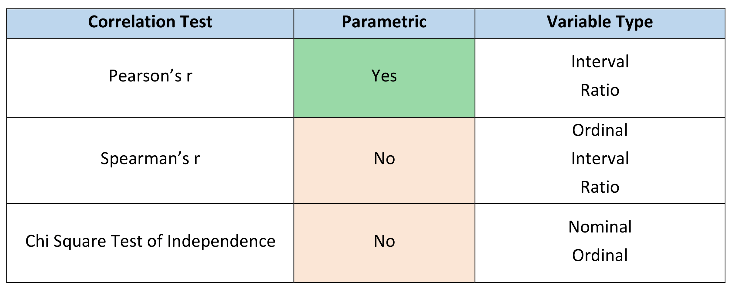
Correlation Test
These assess the extent to which two variables are associated without assuming cause-and-effect relationships. The tests you can employ depend upon whether the data is parametric and the levels of measurement of your variables. The tests are as follows:
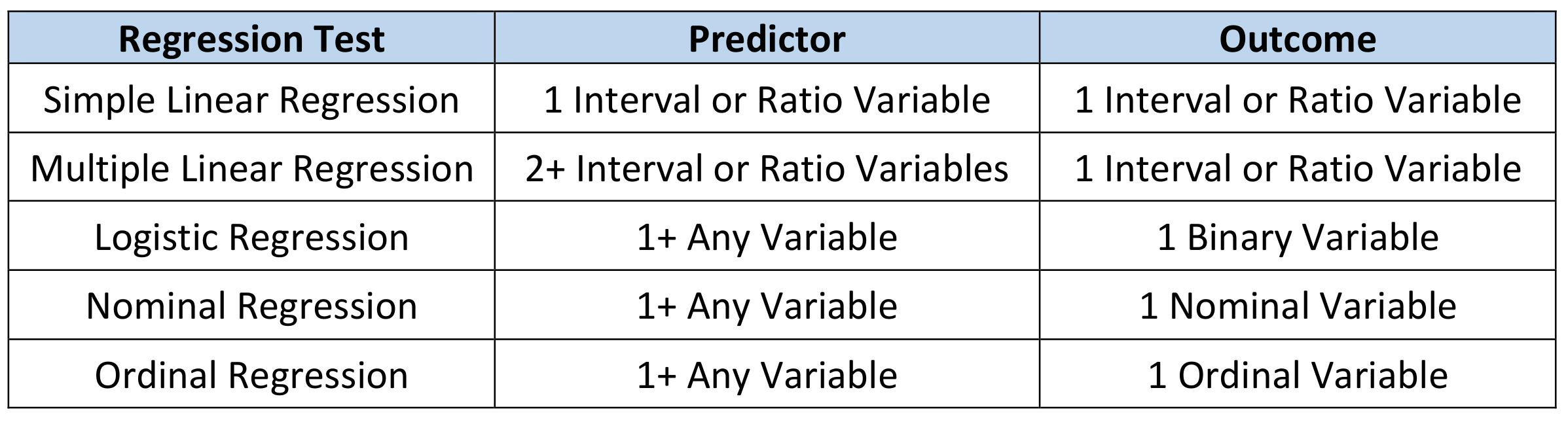
Regression Tests
These demonstrate whether changes in predictor variables causes changes in an outcome variable. They are used to test cause-and-effect relationships. The choice of test will depend upon the number and types of variables you have as predictors and outcomes. These tests use parametric data. If your data is not normally distributed, you can perform data transformations before using them. The tests are as follows: