Introduction to Descriptive Statistics

Descriptive statistics is the term given to the descriptive analysis or summary of data. It can be used in a meaningful way to help identify patterns from within the data. Descriptive statistics are not able to draw conclusions beyond the analysed data and cannot be used to make conclusions on any hypotheses. The main benefit of descriptive statistics is the ability to present the gathered data in a meaningful way to enable simpler interpretation. This article explores the fundamentals of descriptive statistics. You can read about the basics of inferential statistics in our other article.

Data Types and Levels of Measurement

It is essential to understand the nature of your data and how it was measured before you decide which descriptive statistical method to employ. The data will also have implications for which type of inferential statistics is most appropriate for interpretation. This section describes the different data types you will encounter and the various scales of measurement they might use.

Data Types

Most data falls into one of two groups:

Categorical (Qualitative) Data

Data that represents categories.

Numerical (Quantitative) Data

Data that is counted or measured using a numerically defined method.

Numerical data can be further divided into two data types:

Discrete Data: This is numerical data for observations that can only take certain numerical values. This can be finite (fixed number of possible values) or infinite. An example is the number of patients in a clinic.

Continuous Data: This is numerical data that could theoretically be measured in infinitely small units within a given range. An example is the exact volume of water in a bath.

Levels of Measurement

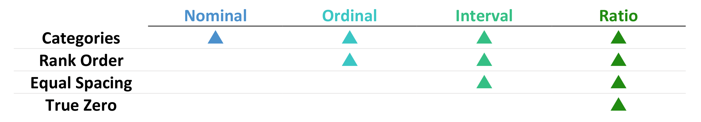
Also known as scales of measurement, these tell you how precisely variables are recorded. There are four levels of measurement and they are described below from lowest to highest precision.

Nominal

This data can only be categorised. Data is given mutually exclusive labels and there is no order between categories. An example is car brands.

Ordinal

This data can be categorised and ranked. You cannot say anything about the intervals between the rankings. An example is language ability.

Interval

This data can be categorised, ranked and evenly spaced. There is no true zero point with different scales giving different zero points. An example is temperature in Fahrenheit or Celsius.

Raio

This data can be categorised, ranked, evenly spaced and has a true zero point. An example is temperature in Kelvin.

Descriptive Analysis

Descriptive statistics is used to summarise and organise characteristics of a data set. There are three main types of descriptive statistics. They are distribution, central tendency and variability. Each type of descriptive statistics can be used on one variable at a time (univariate analysis), with two variables (bivariate analysis) or across more than two variables (multivariate analysis). Each type of descriptive statistics is covered in the following below.

Distribution

A dataset is comprised of a distribution of values. You can summarise the frequency of every possible value in numbers or percentages by creating a frequency distribution table. For categorical data, list each category and count the number of occurrences within each. For numerical data, separate the data into defined interval sizes and count the number of occurrences within each interval (create a histogram plot). Distributions can be symmetrically or asymmetrically distributed.

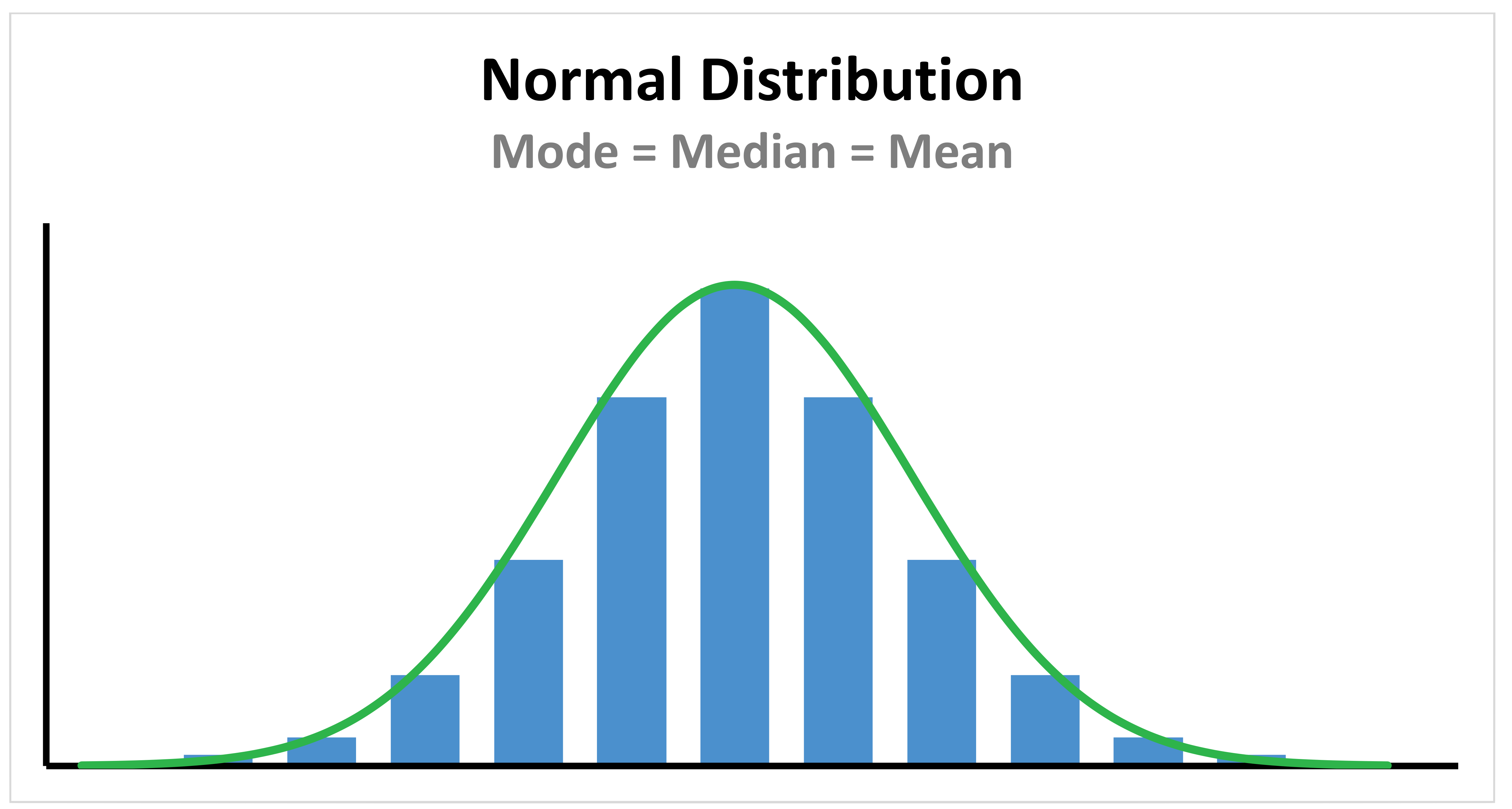
Normal Distribution (Gaussian)

Data is symmetrically distributed with most values clustering around a central region. The mean, mode and median are exactly the same in a normal distribution. Normal distributions have the characteristic symmetrical ‘bell-shape’. The height and width of the distribution is controlled by the central tendency and the variability.

Introducing Z-Scores. A standard normal distribution (z-Distribution) is a normal distribution with a mean of 0 and a standard deviation of 1. Any point (x) from any normal distribution can be converted to the standard normal distribution with the following formula:

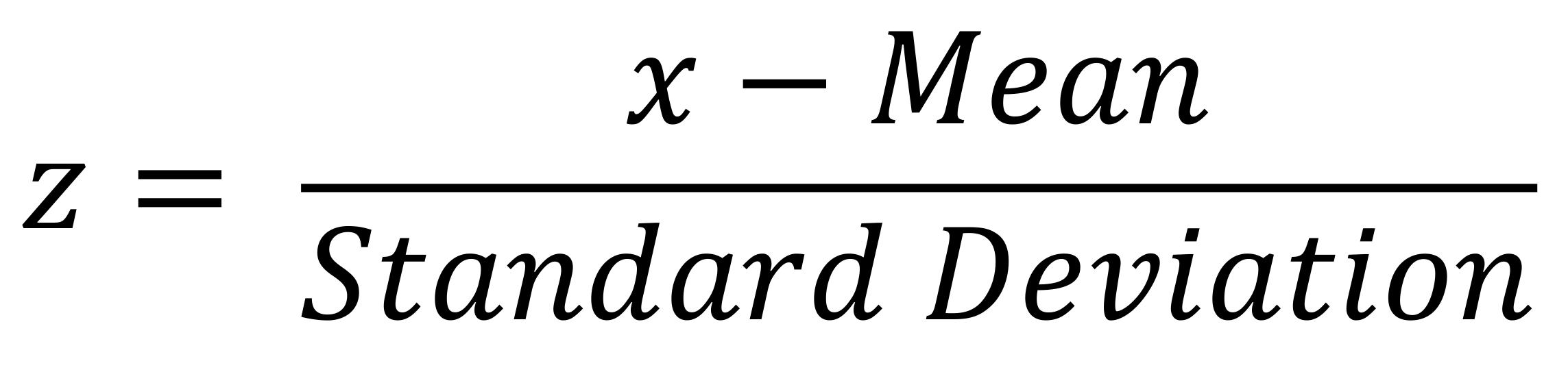
Where z represents the number of standard deviations (distance) value x is from the sample or population mean. These scores are useful for putting data from different sources onto the same scale.

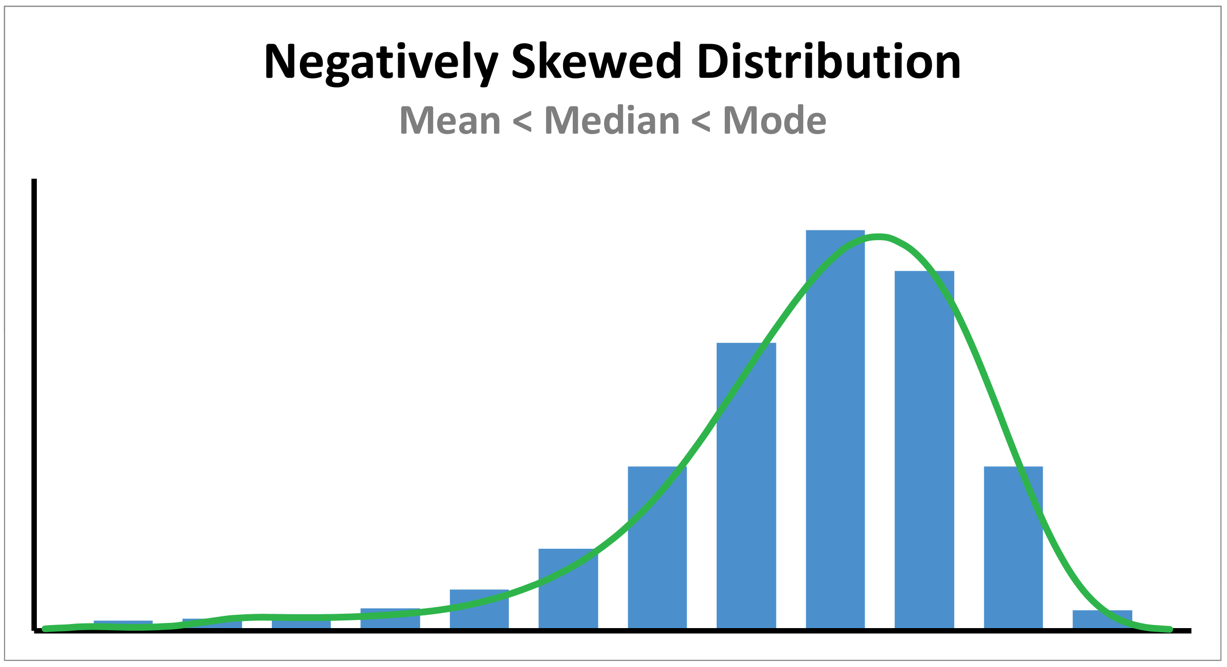
Skewed Distribution

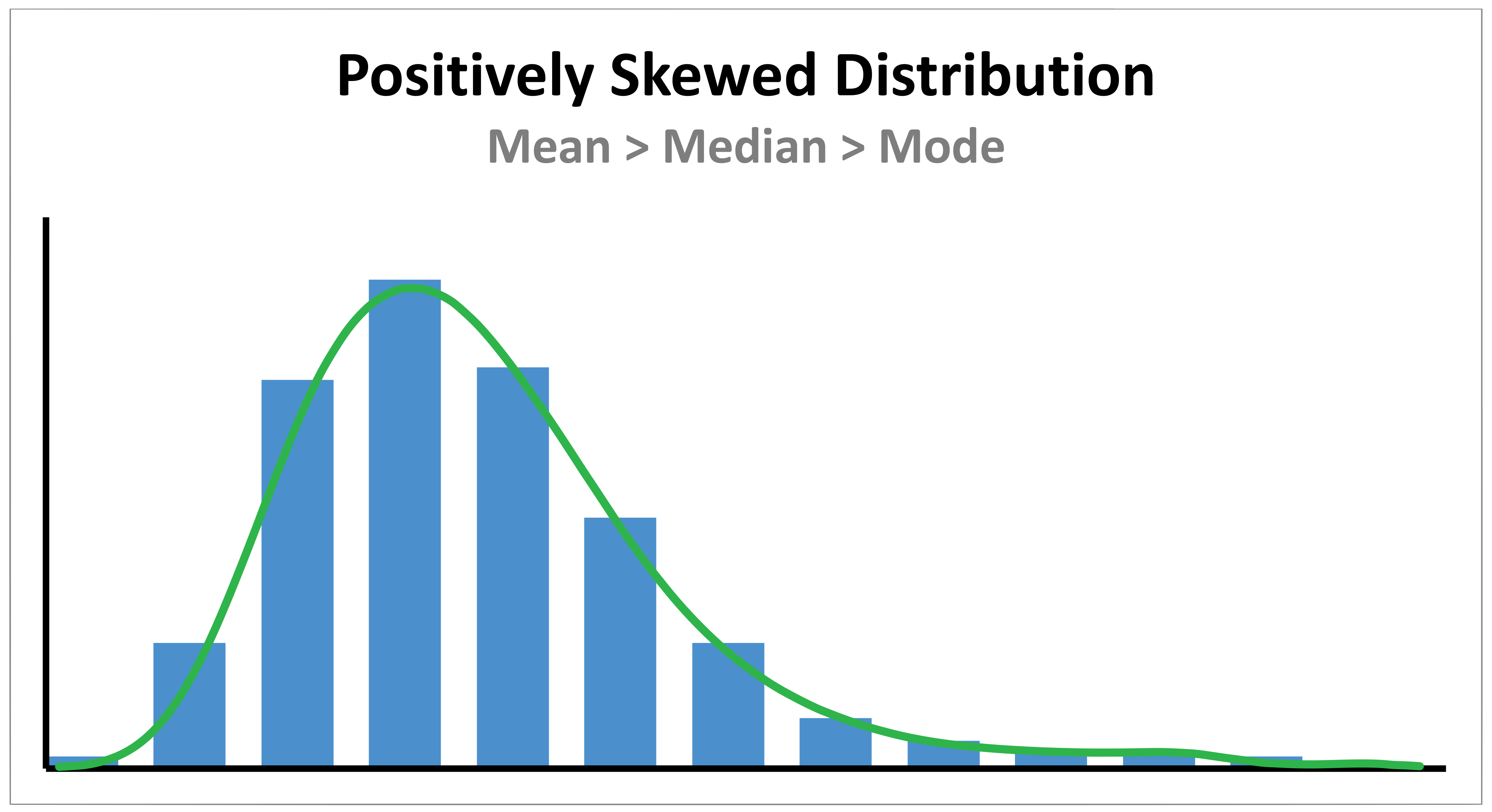
Skewness describes the asymmetry of a distribution. Data is asymmetrical distributed with most values falling on one side of the centre than the other. The mean, median and mode all differ from each other. Positively skewed distributions are more common than negatively skewed ones.

A positively skewed distribution has a cluster of lower scores and a spread-out tail on the right. Here the Mean > Median > Mode.

A negatively skewed distribution has a cluster of higher scores and a spread-out tail on the left. Here the Mean < Median < Mode.

Measures of Central Tendency

These estimate the centre of a dataset. There are three main methods for finding the centre; they are the mean, median and mode. In a perfectly symmetrical, non-skewed distribution, all three are equal.

Mode

This is the most commonly occurring value in a distribution. A data set can have no mode, one mode or more than one mode. The mode can be used for any level of measurement (i.e. nominal, ordinal, interval or ratio levels of measurement) but is most applicable to data with a nominal level of measurement (i.e. data that can only be categorised into mutually exclusive categories).

Median

This is the middle value in a sorted distribution (sorted smallest to largest). When there is an even number of observations, the median is the mean of the two central values. The median can only be used on data that can be ordered (i.e. ordinal, interval or ratio levels of measurement).

Mean

This is the average (sum of observations divided by number of observations) within a distribution. Outliers can significantly increase or decrease the mean when they are included in the calculation. The mean can only be used on data with equal spacing between adjacent values (i.e. interval or ratio levels of measurement).

A word on population mean vs. sample mean. A population is the entire group you are interested in researching, while a sample is only a subset of that population. Data form a sample can help you make estimates, but only the full population data will give you the complete picture. The notation used for these two measures is different, but the calculation is the same.

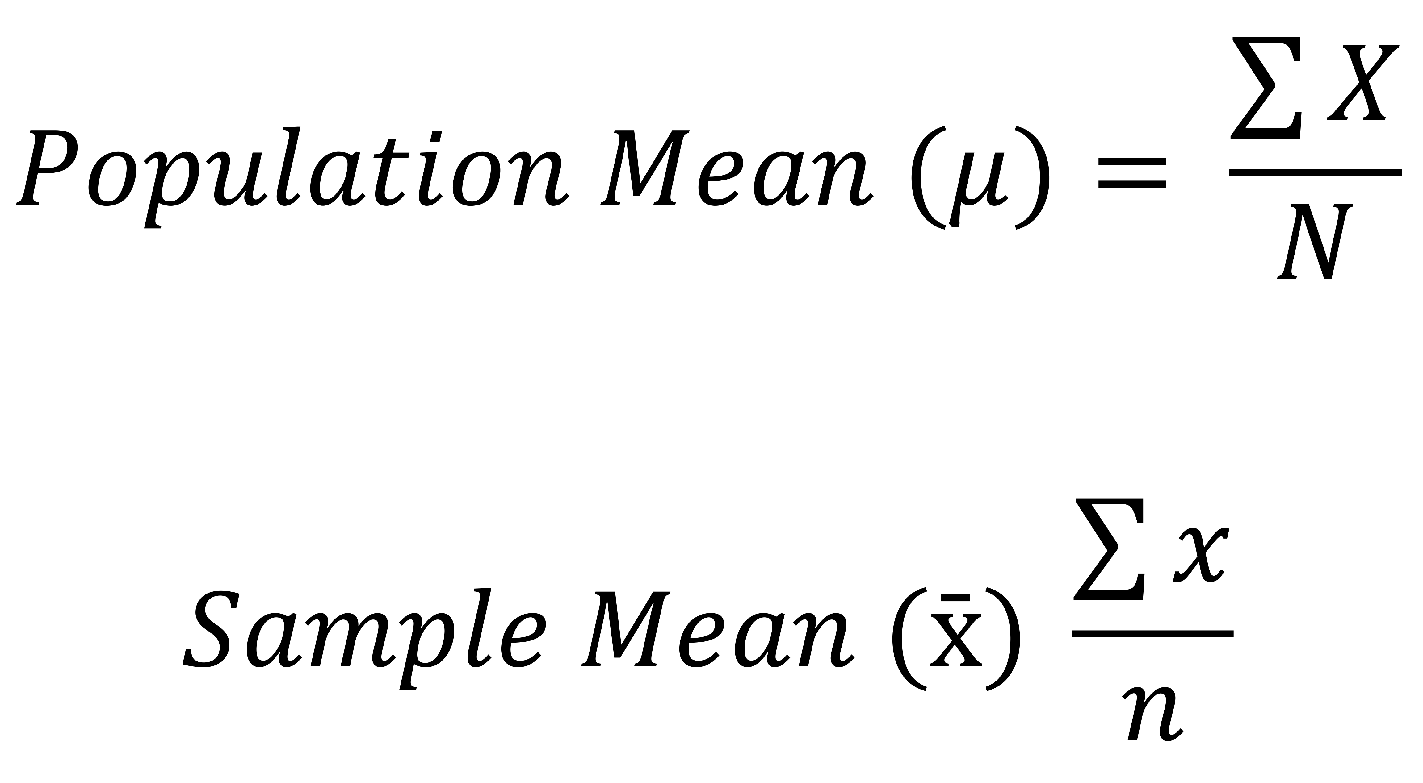
Where μ is the population mean and x̄ is the sample mean. Note how N refers to the number of values in the population data, whereas n refers to the number of values in the sample data. Similarly, X refers to the values in the population data, whereas x refers to the values in the sample data.

Measures of Variability

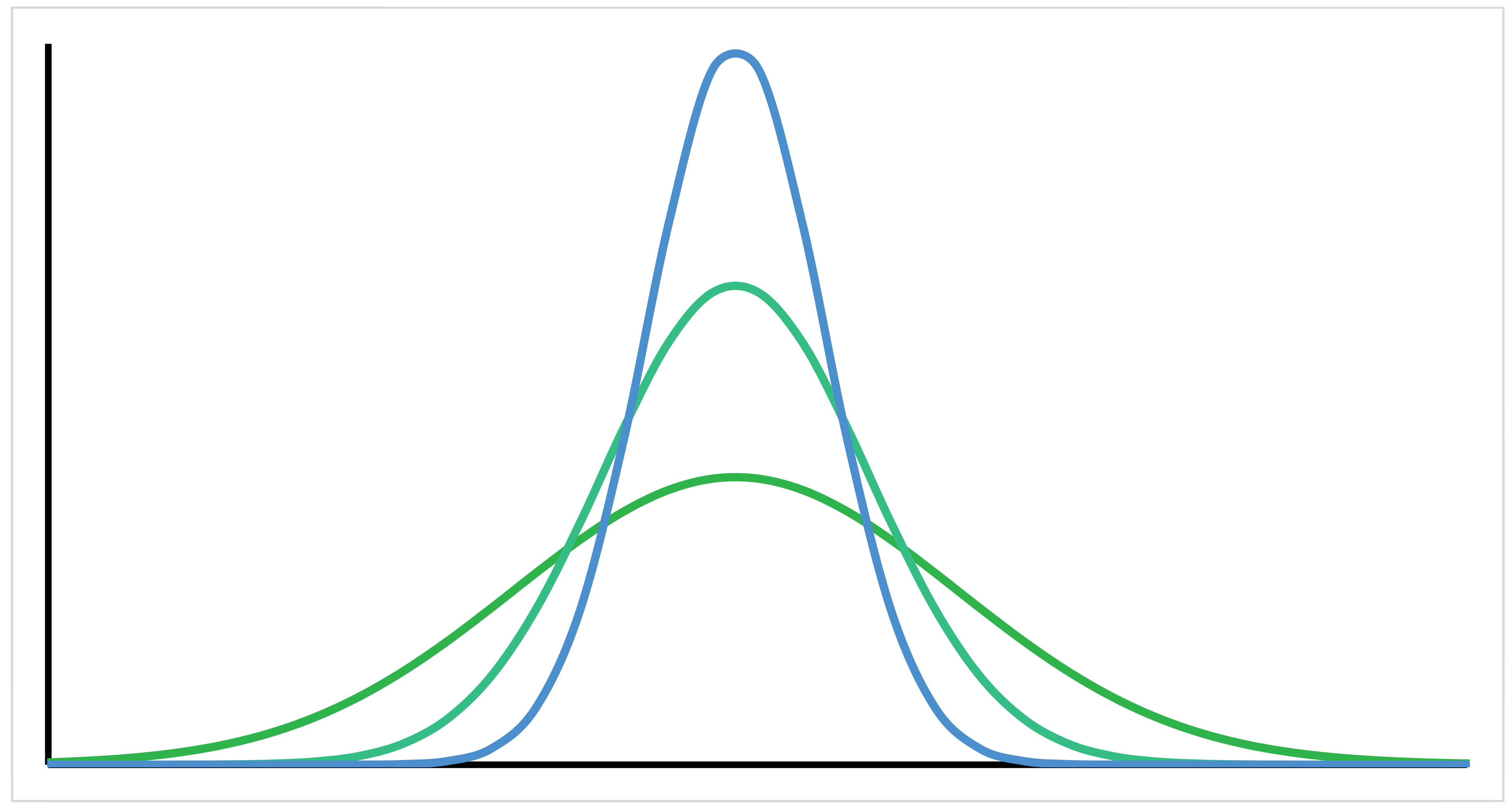
Variability describes how far data points lie from each other and from the centre of a distribution. Low variability (i.e. data is clustered around the centre) helps make better predictions about the population from a sample. Variability can be reflected in four measurements: the range, the interquartile range, standard deviation and variance. In the following diagram there are three example normal distributions. Each line has the same area under the curve and the same mean. However, the variability within each data set is different. The taller curves have a smaller variability.

Range

This is the lowest value subtracted from the highest value. It gives you an idea of how far apart the most extreme responses are. The range is influenced by outliers and doesn’t give you information about the distribution of values. It is best used in combination with other measures and is a good indicator of variability when you have a distribution without extreme values.

Along with the interquartile range, these are the only measures of variability that can be used with ordinal data.

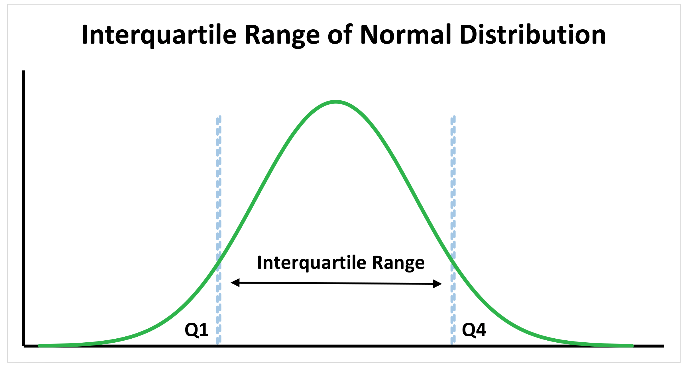
Interquartile Range

This gives you the spread of the middle of your distribution. For any distribution that is ordered from low to high, the interquartile range contains half the values. It is calculated as the third quartile minus the first quartile using either the inclusive or exclusive methods. It is less affected by outliers as the values used to calculate are taken from the middle half of the dataset. It works well with both normal distributions and skewed distributions.

The interquartile range is the best measure for skewed distributions as it is least affected by outliers and focuses on the spread in the middle of the dataset.

Along with the range, these are the only measures of variability that can be used with ordinal data.

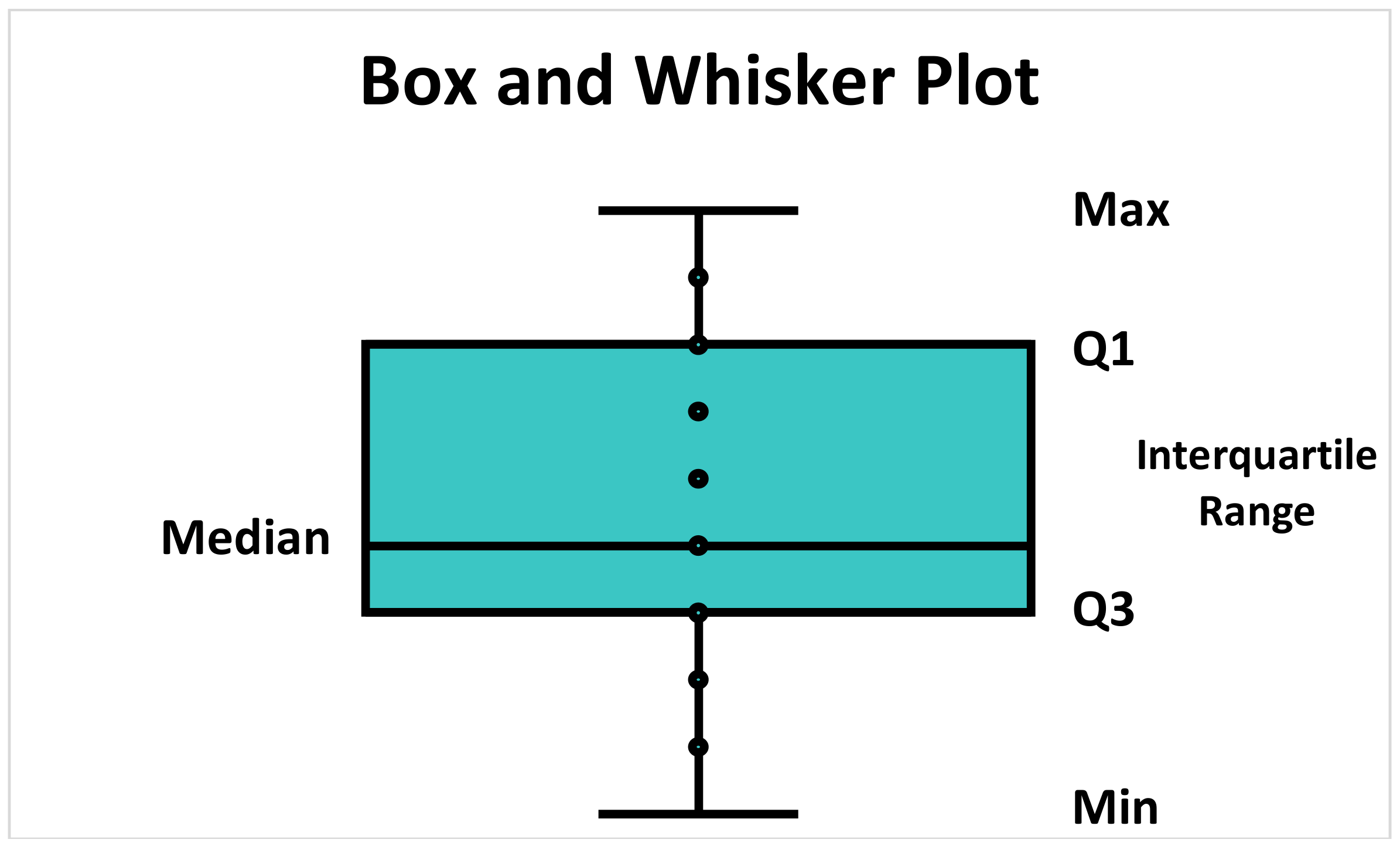
A quick introduction to the five-number summary. This can be used to encapsulate the range and interquartile range. It can be visualised using a box and whisker plot. It includes:

Lowest Value
Q1: 25th percentile
Q2: The median
Q3: 75th percentile
Highest Value

The placement of the box tells you the direction of a skew, if any is present. A box closer to the right (or bottom) means a negatively skewed distribution, while a box closer to the left (or top) means a positively skewed distribution.

Standard Deviation

This is the average amount of variability in your dataset, and it tells you, on average, how far each score lies from the mean. The larger the standard deviation, the more variable the dataset and the further each value, on average, lies from the mean. It is a useful measure of spread for normal distributions. It is less reliable for non-normal distributions and should be used in combination with other measures such as the range or interquartile range in these cases. It is found using the following formulas:

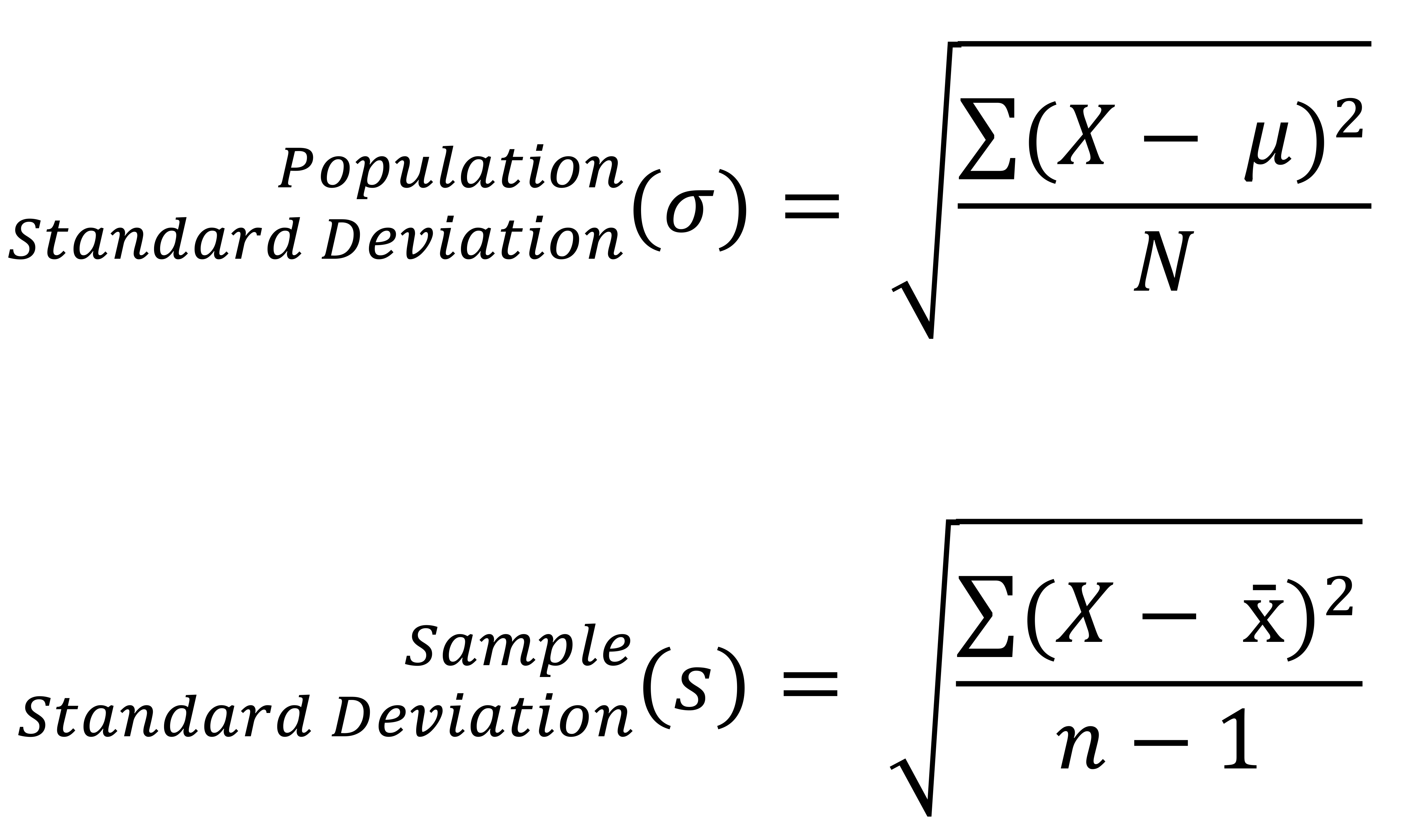
Where σ is the population standard deviation and s is the sample standard deviation. Note how N refers to the number of values in the population data, whereas n refers to the number of values in the sample data. Similarly, μ refers to the mean of the population data, whereas x̄ refers to the mean of the sample data.

Bias and Standard Deviation in Sample Calculations: The use of n - 1 in sample calculations is to make the standard deviation artificially large, giving you a conservative estimate of variability (overestimate). While not unbiased (due to the square root function), it is less biased as an estimate than when n is used alone (this would underestimate variability in samples).

Standard Deviation and Normal Distributions: If used within a normal distribution, the standard deviation and the mean will tell you where most the values within your distribution lie:

68% of scores are within 2 standard deviations of the mean.
95% of scores are within 4 standard deviations of the mean.
99.7% of scores are within 6 standard deviations of the mean.

Variance

This is the average of squared deviations from the mean. It reflects the degree of spread in the dataset. The larger the variance in relation to the mean, the more spread the data. It is calculated by squaring the standard deviation or using the following formulas:

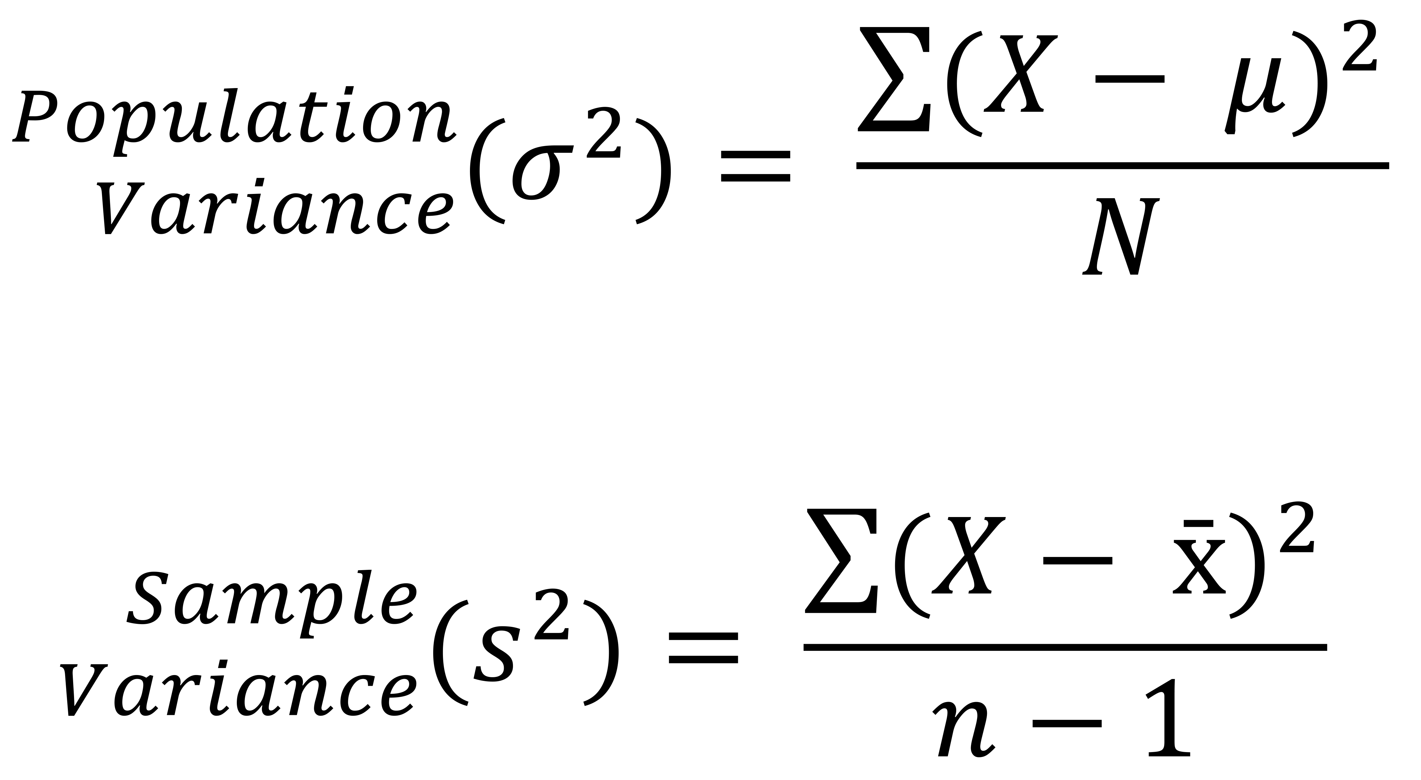
Where σ^2 is the population variance and s^2 is the sample variance. Note how N refers to the number of values in the population data, whereas n refers to the number of values in the sample data. Similarly, μ refers to the mean of the population data, whereas x̄ refers to the mean of the sample data.

Removal of Bias from Sample Variance Calculations: Note that the use of n - 1 in sample calculations is to make the variance artificially large (overestimate). This removes the bias that would be seen where n used alone (this would be biased towards underestimating variability).

Statistical Relevance of Variance: Variance is important for parametrical statistical testing as they require similar or equal variances between samples. If there is a difference in variances, samples can be compared (i.e. use ANOVA testing) to ascertain whether these differences are due to samples being drawn from different populations or as a result of sample variation.

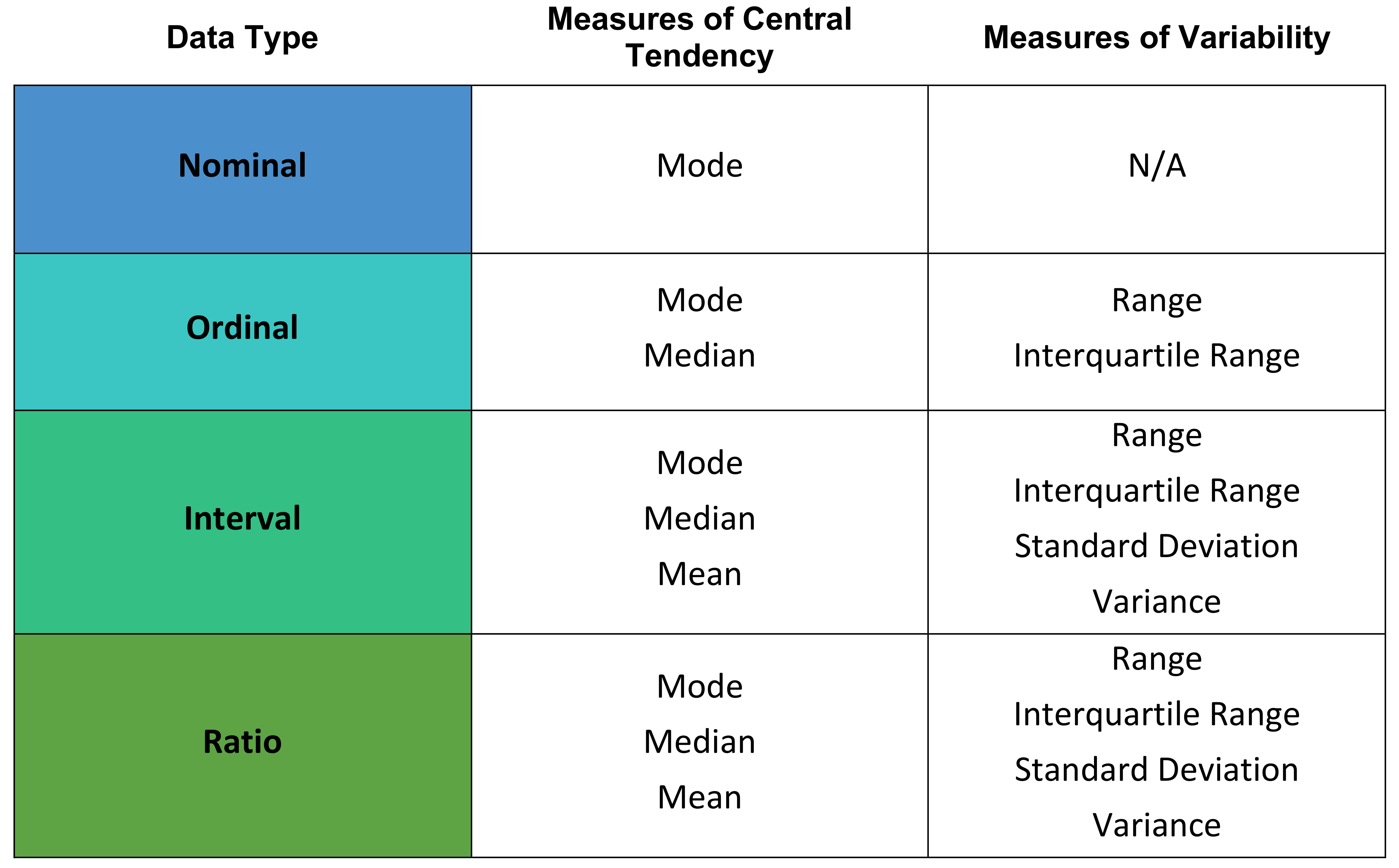
Summary of Descriptive Statistics

The following table provides a summary of how the level of measurement relates to the central tendancy and the variability.